Category: pro
Python hosting: Host, run, and code Python in the cloud!
Matplotlib Histogram
Matplotlib can be used to create histograms. A histogram shows the frequency on the vertical axis and the horizontal axis is another dimension. Usually it has bins, where every bin has a minimum and maximum value. Each bin also has a frequency between x and infinite.
Related course
Matplotlib histogram example
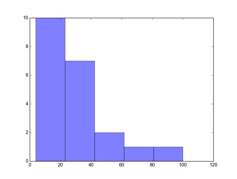
Below we show the most minimal Matplotlib histogram:
import numpy as np import matplotlib.mlab as mlab import matplotlib.pyplot as plt x = [21,22,23,4,5,6,77,8,9,10,31,32,33,34,35,36,37,18,49,50,100] num_bins = 5 n, bins, patches = plt.hist(x, num_bins, facecolor='blue', alpha=0.5) plt.show() |
Output:
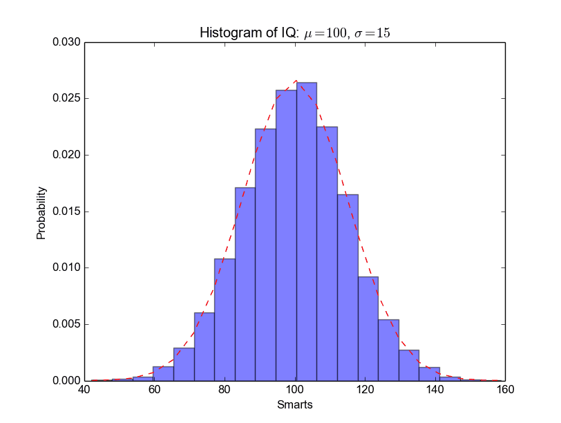
A complete matplotlib python histogram
Many things can be added to a histogram such as a fit line, labels and so on. The code below creates a more advanced histogram.
#!/usr/bin/env python import numpy as np import matplotlib.mlab as mlab import matplotlib.pyplot as plt # example data mu = 100 # mean of distribution sigma = 15 # standard deviation of distribution x = mu + sigma * np.random.randn(10000) num_bins = 20 # the histogram of the data n, bins, patches = plt.hist(x, num_bins, normed=1, facecolor='blue', alpha=0.5) # add a 'best fit' line y = mlab.normpdf(bins, mu, sigma) plt.plot(bins, y, 'r--') plt.xlabel('Smarts') plt.ylabel('Probability') plt.title(r'Histogram of IQ: $\mu=100$, $\sigma=15$') # Tweak spacing to prevent clipping of ylabel plt.subplots_adjust(left=0.15) plt.show() |
Output:
Matplotlib Line chart
A line chart can be created using the Matplotlib plot() function. While we can just plot a line, we are not limited to that. We can explicitly define the grid, the x and y axis scale and labels, title and display options.
Related course:
Line chart example
The example below will create a line chart.
from pylab import * t = arange(0.0, 2.0, 0.01) s = sin(2.5*pi*t) plot(t, s) xlabel('time (s)') ylabel('voltage (mV)') title('Sine Wave') grid(True) show() |
Output:
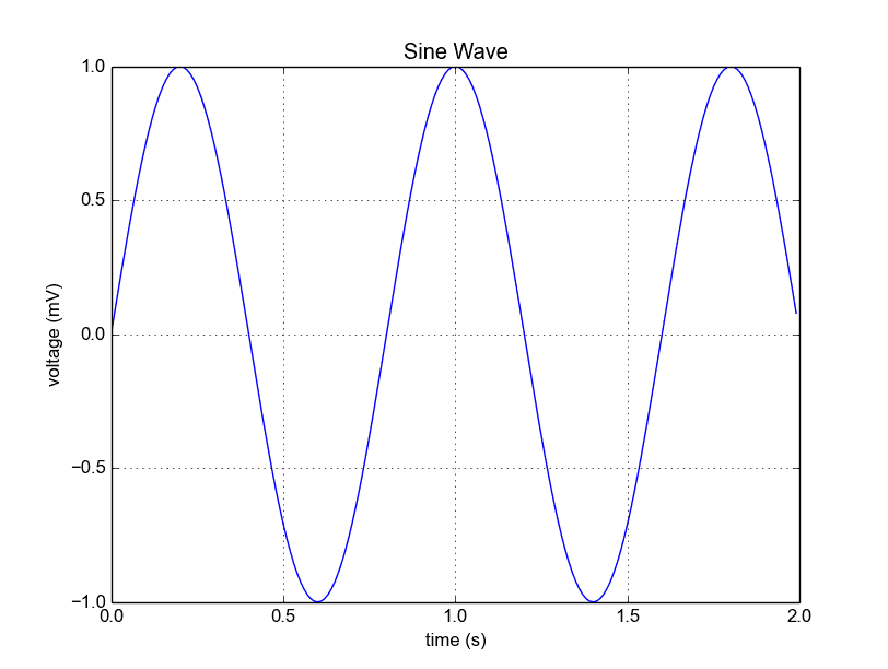
The lines:
from pylab import * t = arange(0.0, 2.0, 0.01) s = sin(2.5*pi*t) |
simply define the data to be plotted.
from pylab import * t = arange(0.0, 2.0, 0.01) s = sin(2.5*pi*t) plot(t, s) show() |
plots the chart. The other statements are very straightforward: statements xlabel() sets the x-axis text, ylabel() sets the y-axis text, title() sets the chart title and grid(True) simply turns on the grid.
If you want to save the plot to the disk, call the statement:
savefig("line_chart.png") |
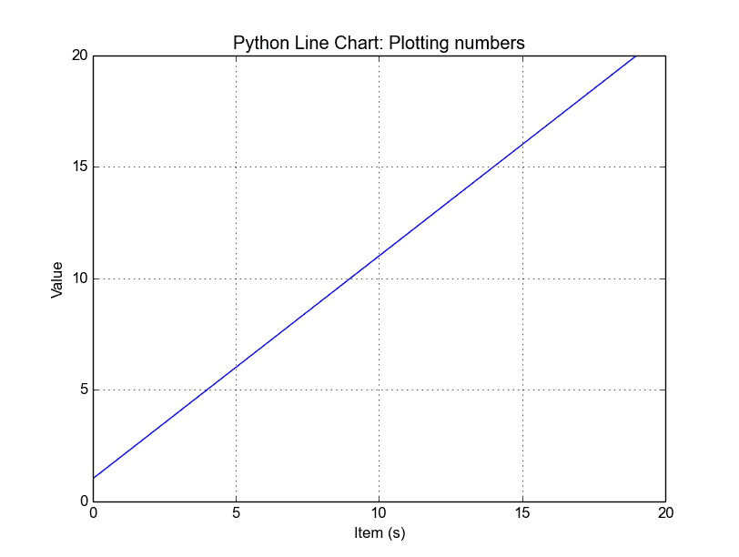
Plot a custom Line Chart
If you want to plot using an array (list), you can execute this script:
from pylab import * t = arange(0.0, 20.0, 1) s = [1,2,3,4,5,6,7,8,9,10,11,12,13,14,15,16,17,18,19,20] plot(t, s) xlabel('Item (s)') ylabel('Value') title('Python Line Chart: Plotting numbers') grid(True) show() |
The statement:
t = arange(0.0, 20.0, 1) |
defines start from 0, plot 20 items (length of our array) with steps of 1.
Output:
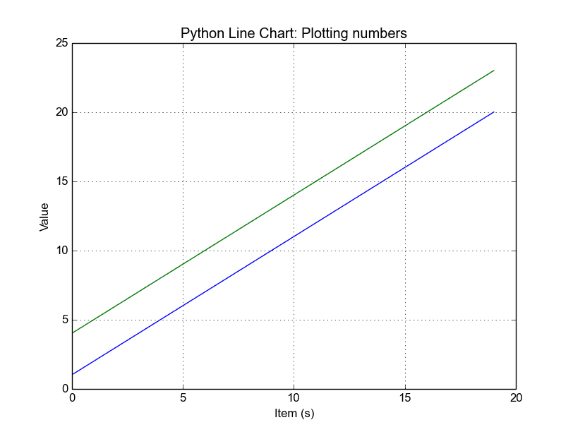
Multiple plots
If you want to plot multiple lines in one chart, simply call the plot() function multiple times. An example:
from pylab import * t = arange(0.0, 20.0, 1) s = [1,2,3,4,5,6,7,8,9,10,11,12,13,14,15,16,17,18,19,20] s2 = [4,5,6,7,8,9,10,11,12,13,14,15,16,17,18,19,20,21,22,23] plot(t, s) plot(t, s2) xlabel('Item (s)') ylabel('Value') title('Python Line Chart: Plotting numbers') grid(True) show() |
Output:
In case you want to plot them in different views in the same window you can use this:
import matplotlib.pyplot as plt from pylab import * t = arange(0.0, 20.0, 1) s = [1,2,3,4,5,6,7,8,9,10,11,12,13,14,15,16,17,18,19,20] s2 = [4,5,6,7,8,9,10,11,12,13,14,15,16,17,18,19,20,21,22,23] plt.subplot(2, 1, 1) plt.plot(t, s) plt.ylabel('Value') plt.title('First chart') plt.grid(True) plt.subplot(2, 1, 2) plt.plot(t, s2) plt.xlabel('Item (s)') plt.ylabel('Value') plt.title('Second chart') plt.grid(True) plt.show() |
Output:
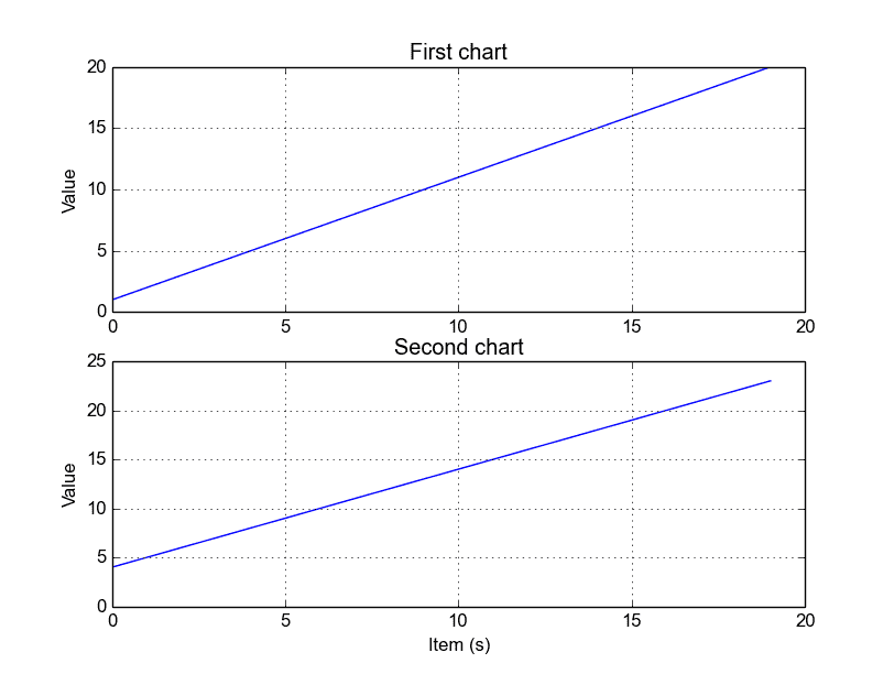
The plt.subplot() statement is key here. The subplot() command specifies numrows, numcols and fignum.
Styling the plot
If you want thick lines or set the color, use:
plot(t, s, color="red", linewidth=2.5, linestyle="-") |
Matplotlib Bar chart
Matplotlib may be used to create bar charts. You might like the Matplotlib gallery.
Related course
The course below is all about data visualization:
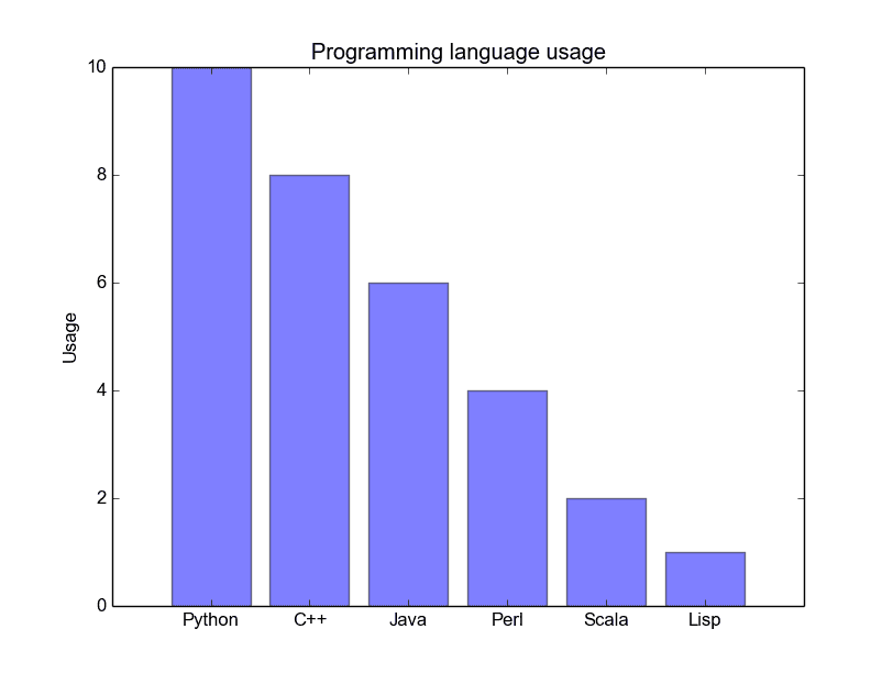
Bar chart code
The code below creates a bar chart:
import matplotlib.pyplot as plt; plt.rcdefaults() import numpy as np import matplotlib.pyplot as plt objects = ('Python', 'C++', 'Java', 'Perl', 'Scala', 'Lisp') y_pos = np.arange(len(objects)) performance = [10,8,6,4,2,1] plt.bar(y_pos, performance, align='center', alpha=0.5) plt.xticks(y_pos, objects) plt.ylabel('Usage') plt.title('Programming language usage') plt.show() |
Output:
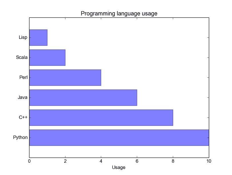
Matplotlib charts can be horizontal, to create a horizontal bar chart:
import matplotlib.pyplot as plt; plt.rcdefaults() import numpy as np import matplotlib.pyplot as plt objects = ('Python', 'C++', 'Java', 'Perl', 'Scala', 'Lisp') y_pos = np.arange(len(objects)) performance = [10,8,6,4,2,1] plt.barh(y_pos, performance, align='center', alpha=0.5) plt.yticks(y_pos, objects) plt.xlabel('Usage') plt.title('Programming language usage') plt.show() |
Output:
More on bar charts
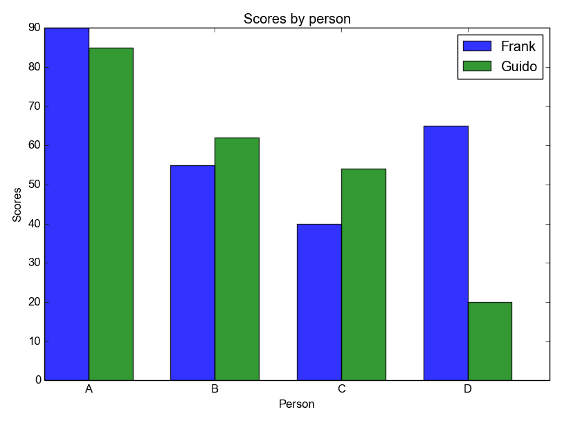
You can compare two data series using this Matplotlib code:
import numpy as np import matplotlib.pyplot as plt # data to plot n_groups = 4 means_frank = (90, 55, 40, 65) means_guido = (85, 62, 54, 20) # create plot fig, ax = plt.subplots() index = np.arange(n_groups) bar_width = 0.35 opacity = 0.8 rects1 = plt.bar(index, means_frank, bar_width, alpha=opacity, color='b', label='Frank') rects2 = plt.bar(index + bar_width, means_guido, bar_width, alpha=opacity, color='g', label='Guido') plt.xlabel('Person') plt.ylabel('Scores') plt.title('Scores by person') plt.xticks(index + bar_width, ('A', 'B', 'C', 'D')) plt.legend() plt.tight_layout() plt.show() |
Output:
Download All Matplotlib Examples
Matplotlib Pie chart
Matplotlib supports pie charts using the pie() function. You might like the Matplotlib gallery.
Related course:
Matplotlib pie chart
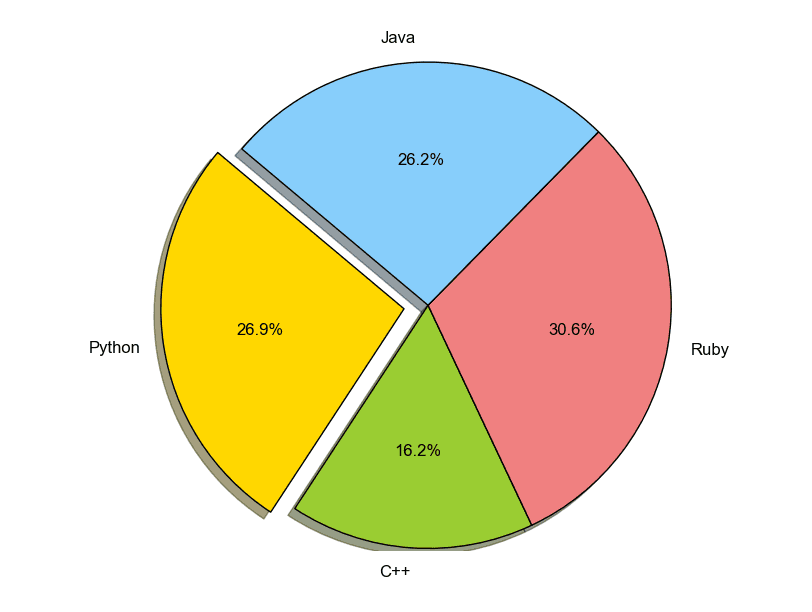
The code below creates a pie chart:
import matplotlib.pyplot as plt # Data to plot labels = 'Python', 'C++', 'Ruby', 'Java' sizes = [215, 130, 245, 210] colors = ['gold', 'yellowgreen', 'lightcoral', 'lightskyblue'] explode = (0.1, 0, 0, 0) # explode 1st slice # Plot plt.pie(sizes, explode=explode, labels=labels, colors=colors, autopct='%1.1f%%', shadow=True, startangle=140) plt.axis('equal') plt.show() |
Output:
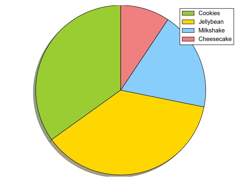
To add a legend use the plt.legend() function:
import matplotlib.pyplot as plt labels = ['Cookies', 'Jellybean', 'Milkshake', 'Cheesecake'] sizes = [38.4, 40.6, 20.7, 10.3] colors = ['yellowgreen', 'gold', 'lightskyblue', 'lightcoral'] patches, texts = plt.pie(sizes, colors=colors, shadow=True, startangle=90) plt.legend(patches, labels, loc="best") plt.axis('equal') plt.tight_layout() plt.show() |
Output:
Download All Matplotlib Examples
Matplotlib legend
Matplotlib has native support for legends. Legends can be placed in various positions: A legend can be placed inside or outside the chart and the position can be moved.
The legend() method adds the legend to the plot. In this article we will show you some examples of legends using matplotlib.
Related course
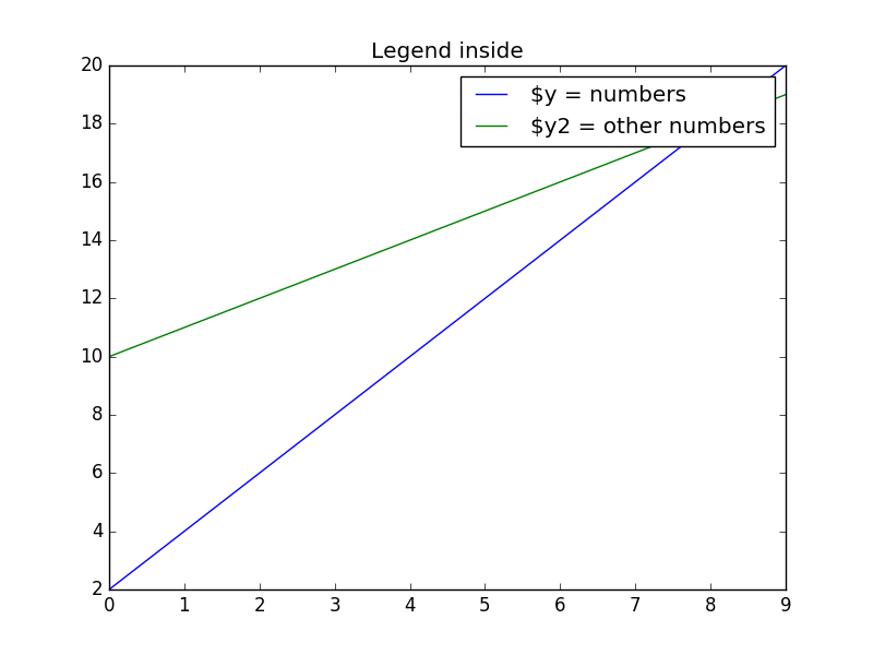
Matplotlib legend inside
To place the legend inside, simply call legend():
import matplotlib.pyplot as plt import numpy as np y = [2,4,6,8,10,12,14,16,18,20] y2 = [10,11,12,13,14,15,16,17,18,19] x = np.arange(10) fig = plt.figure() ax = plt.subplot(111) ax.plot(x, y, label='$y = numbers') ax.plot(x, y2, label='$y2 = other numbers') plt.title('Legend inside') ax.legend() plt.show() |
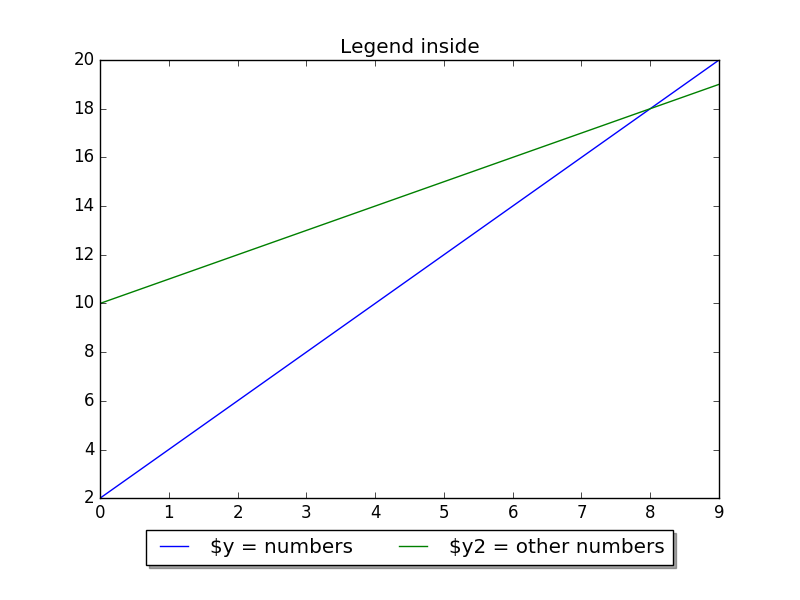
Matplotlib legend on bottom
To place the legend on the bottom, change the legend() call to:
ax.legend(loc='upper center', bbox_to_anchor=(0.5, -0.05), shadow=True, ncol=2) |
Take into account that we set the number of columns two ncol=2 and set a shadow.
The complete code would be:
import matplotlib.pyplot as plt import numpy as np y = [2,4,6,8,10,12,14,16,18,20] y2 = [10,11,12,13,14,15,16,17,18,19] x = np.arange(10) fig = plt.figure() ax = plt.subplot(111) ax.plot(x, y, label='$y = numbers') ax.plot(x, y2, label='$y2 = other numbers') plt.title('Legend inside') ax.legend(loc='upper center', bbox_to_anchor=(0.5, -0.05), shadow=True, ncol=2) plt.show() |
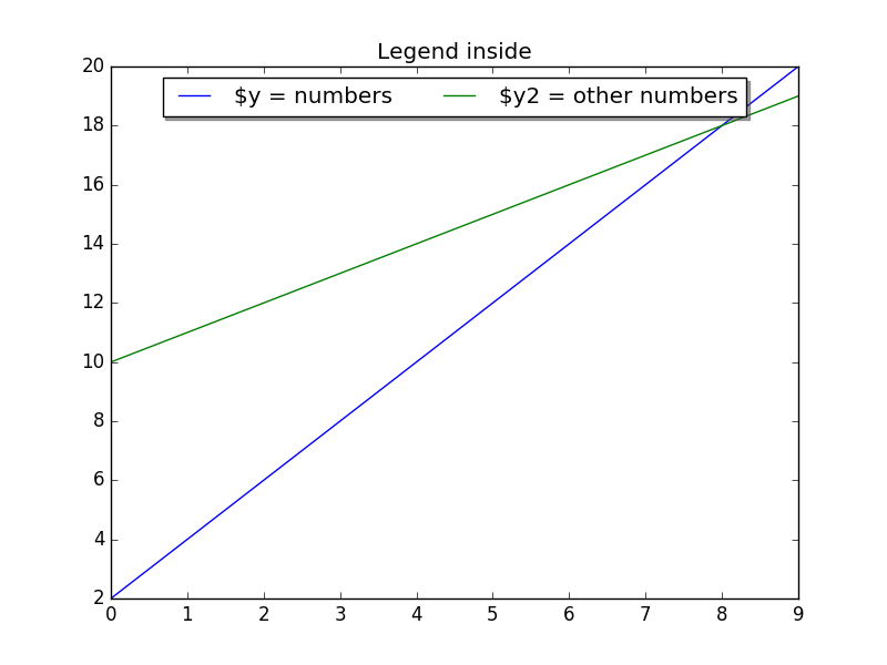
Matplotlib legend on top
To put the legend on top, change the bbox_to_anchor values:
ax.legend(loc='upper center', bbox_to_anchor=(0.5, 1.00), shadow=True, ncol=2) |
Code:
import matplotlib.pyplot as plt import numpy as np y = [2,4,6,8,10,12,14,16,18,20] y2 = [10,11,12,13,14,15,16,17,18,19] x = np.arange(10) fig = plt.figure() ax = plt.subplot(111) ax.plot(x, y, label='$y = numbers') ax.plot(x, y2, label='$y2 = other numbers') plt.title('Legend inside') ax.legend(loc='upper center', bbox_to_anchor=(0.5, 1.00), shadow=True, ncol=2) plt.show() |
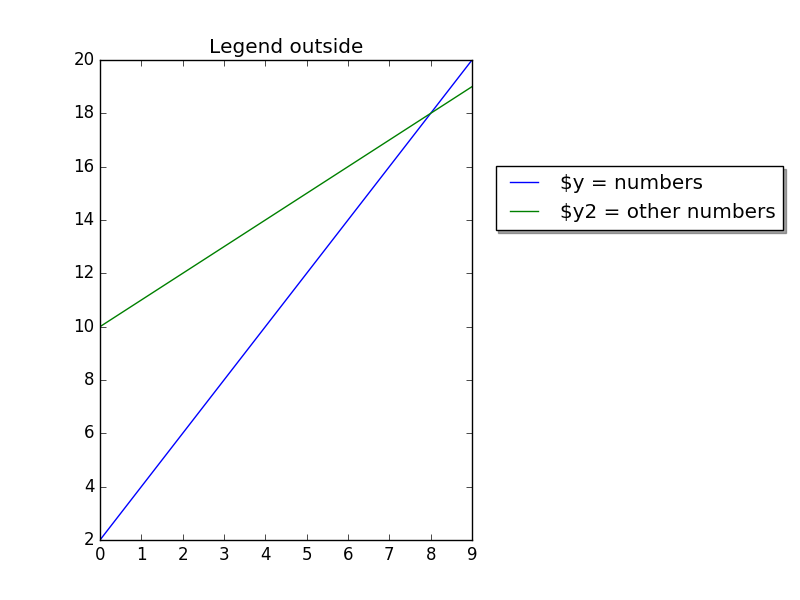
Legend outside right
We can put the legend ouside by resizing the box and puting the legend relative to that:
chartBox = ax.get_position() ax.set_position([chartBox.x0, chartBox.y0, chartBox.width*0.6, chartBox.height]) ax.legend(loc='upper center', bbox_to_anchor=(1.45, 0.8), shadow=True, ncol=1) |
Code:
import matplotlib.pyplot as plt import numpy as np y = [2,4,6,8,10,12,14,16,18,20] y2 = [10,11,12,13,14,15,16,17,18,19] x = np.arange(10) fig = plt.figure() ax = plt.subplot(111) ax.plot(x, y, label='$y = numbers') ax.plot(x, y2, label='$y2 = other numbers') plt.title('Legend outside') chartBox = ax.get_position() ax.set_position([chartBox.x0, chartBox.y0, chartBox.width*0.6, chartBox.height]) ax.legend(loc='upper center', bbox_to_anchor=(1.45, 0.8), shadow=True, ncol=1) plt.show() |
Matplotlib save figure to image file
Related course
The course below is all about data visualization:
Save figure
Matplotlib can save plots directly to a file using savefig().
The method can be used like this:
fig.savefig('plot.png') |
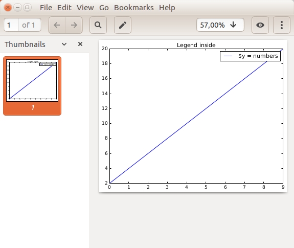
Complete example:
import matplotlib import matplotlib.pyplot as plt import numpy as np y = [2,4,6,8,10,12,14,16,18,20] x = np.arange(10) fig = plt.figure() ax = plt.subplot(111) ax.plot(x, y, label='$y = numbers') plt.title('Legend inside') ax.legend() #plt.show() fig.savefig('plot.png') |
To change the format, simply change the extension like so:
fig.savefig('plot.pdf') |
You can open your file using
display plot.png |
or open it in an image or pdf viewer,