
Category: machine-learning
Python hosting: Host, run, and code Python in the cloud!
k nearest neighbors
Computers can automatically classify data using the k-nearest-neighbor algorithm.
For instance: given the sepal length and width, a computer program can determine if the flower is an Iris Setosa, Iris Versicolour or another type of flower.
Related courses
Dataset
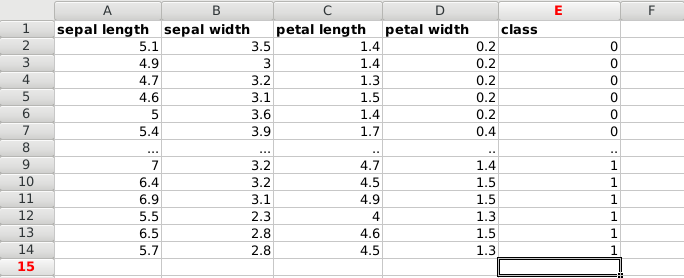
We start with data, in this case a dataset of plants.
Each plant has unique features: sepal length, sepal width, petal length and petal width. The measurements of different plans can be taken and saved into a spreadsheet.
The type of plant (species) is also saved, which is either of these classes:
- Iris Setosa (0)
- Iris Versicolour (1)
- Iris Virginica (2)
Put it all together, and we have a dataset:
We load the data. This is a famous dataset, it’s included in the module. Otherwise you can load a dataset using python pandas.
import matplotlib matplotlib.use('GTKAgg') import numpy as np import matplotlib.pyplot as plt from matplotlib.colors import ListedColormap from sklearn import neighbors, datasets # import some data to play with iris = datasets.load_iris() # take the first two features X = iris.data[:, :2] y = iris.target print(X) |
X contains the first two features, being the rows sepal length and sepal width. The Y list contains the classes for the features.
Plot data
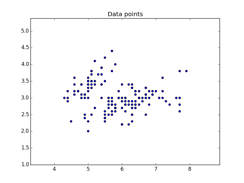
We will use the two features of X to create a plot. Where we use X[:,0] on one axis and X[:,1] on the other.
import matplotlib matplotlib.use('GTKAgg') import numpy as np import matplotlib.pyplot as plt from matplotlib.colors import ListedColormap from sklearn import neighbors, datasets # import some data to play with iris = datasets.load_iris() # take the first two features X = iris.data[:, :2] y = iris.target h = .02 # step size in the mesh # Calculate min, max and limits x_min, x_max = X[:, 0].min() - 1, X[:, 0].max() + 1 y_min, y_max = X[:, 1].min() - 1, X[:, 1].max() + 1 xx, yy = np.meshgrid(np.arange(x_min, x_max, h), np.arange(y_min, y_max, h)) # Put the result into a color plot plt.figure() plt.scatter(X[:, 0], X[:, 1]) plt.xlim(xx.min(), xx.max()) plt.ylim(yy.min(), yy.max()) plt.title("Data points") plt.show() |
This will output the data:
Classify with k-nearest-neighbor
We can classify the data using the kNN algorithm. We create and fit the data using:
clf = neighbors.KNeighborsClassifier(n_neighbors, weights='distance') clf.fit(X, y) |
And predict the class using
clf.predict() |
This gives us the following code:
import matplotlib matplotlib.use('GTKAgg') import numpy as np import matplotlib.pyplot as plt from matplotlib.colors import ListedColormap from sklearn import neighbors, datasets n_neighbors = 6 # import some data to play with iris = datasets.load_iris() # prepare data X = iris.data[:, :2] y = iris.target h = .02 # Create color maps cmap_light = ListedColormap(['#FFAAAA', '#AAFFAA','#00AAFF']) cmap_bold = ListedColormap(['#FF0000', '#00FF00','#00AAFF']) # we create an instance of Neighbours Classifier and fit the data. clf = neighbors.KNeighborsClassifier(n_neighbors, weights='distance') clf.fit(X, y) # calculate min, max and limits x_min, x_max = X[:, 0].min() - 1, X[:, 0].max() + 1 y_min, y_max = X[:, 1].min() - 1, X[:, 1].max() + 1 xx, yy = np.meshgrid(np.arange(x_min, x_max, h), np.arange(y_min, y_max, h)) # predict class using data and kNN classifier Z = clf.predict(np.c_[xx.ravel(), yy.ravel()]) # Put the result into a color plot Z = Z.reshape(xx.shape) plt.figure() plt.pcolormesh(xx, yy, Z, cmap=cmap_light) # Plot also the training points plt.scatter(X[:, 0], X[:, 1], c=y, cmap=cmap_bold) plt.xlim(xx.min(), xx.max()) plt.ylim(yy.min(), yy.max()) plt.title("3-Class classification (k = %i)" % (n_neighbors)) plt.show() |
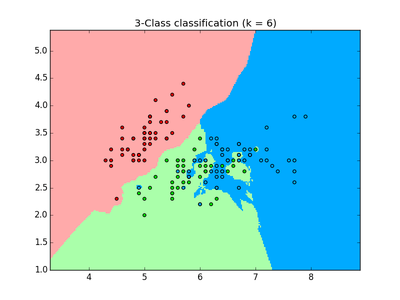
which outputs the plot using the 3 classes:
Prediction
We can use this data to make predictions. Given the position on the plot (which is determined by the features), it’s assigned a class. We can put a new data on the plot and predict which class it belongs to.
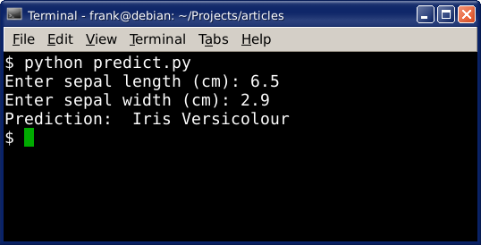
The code below will make prediction based on the input given by the user:
import numpy as np from sklearn import neighbors, datasets from sklearn import preprocessing n_neighbors = 6 # import some data to play with iris = datasets.load_iris() # prepare data X = iris.data[:, :2] y = iris.target h = .02 # we create an instance of Neighbours Classifier and fit the data. clf = neighbors.KNeighborsClassifier(n_neighbors, weights='distance') clf.fit(X, y) # make prediction sl = raw_input('Enter sepal length (cm): ') sw = raw_input('Enter sepal width (cm): ') dataClass = clf.predict([[sl,sw]]) print('Prediction: '), if dataClass == 0: print('Iris Setosa') elif dataClass == 1: print('Iris Versicolour') else: print('Iris Virginica') |
Example output:
Linear Regression
How does regression relate to machine learning?
Given data, we can try to find the best fit line. After we discover the best fit line, we can use it to make predictions.
Consider we have data about houses: price, size, driveway and so on. You can download the dataset for this article here.
Data can be any data saved from Excel into a csv format, we will use Python Pandas to load the data.
Related courses
Required modules
You shoud have a few modules installed:
sudo pip install sklearn sudo pip install scipy sudo pip install scikit-learn |
Load dataset and plot
You can choose the graphical toolkit, this line is optional:
matplotlib.use('GTKAgg') |
We start by loading the modules, and the dataset. Without data we can’t make good predictions.
The first step is to load the dataset. The data will be loaded using Python Pandas, a data analysis module. It will be loaded into a structure known as a Panda Data Frame, which allows for each manipulation of the rows and columns.
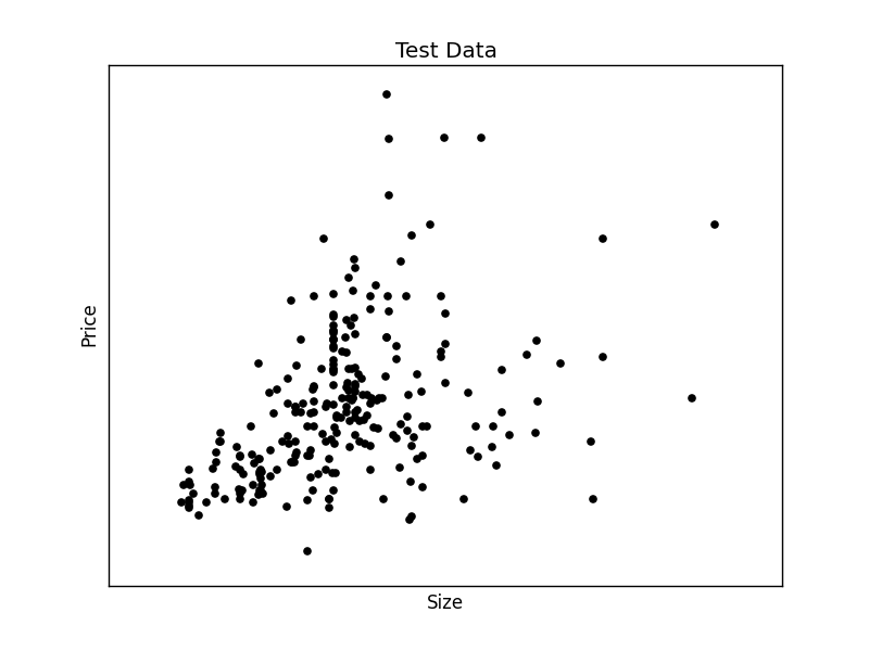
We create two arrays: X (size) and Y (price). Intuitively we’d expect to find some correlation between price and size.
The data will be split into a trainining and test set. Once we have the test data, we can find a best fit line and make predictions.
import matplotlib matplotlib.use('GTKAgg') import matplotlib.pyplot as plt import numpy as np from sklearn import datasets, linear_model import pandas as pd # Load CSV and columns df = pd.read_csv("Housing.csv") Y = df['price'] X = df['lotsize'] X=X.reshape(len(X),1) Y=Y.reshape(len(Y),1) # Split the data into training/testing sets X_train = X[:-250] X_test = X[-250:] # Split the targets into training/testing sets Y_train = Y[:-250] Y_test = Y[-250:] # Plot outputs plt.scatter(X_test, Y_test, color='black') plt.title('Test Data') plt.xlabel('Size') plt.ylabel('Price') plt.xticks(()) plt.yticks(()) plt.show() |
Finally we plot the test data.
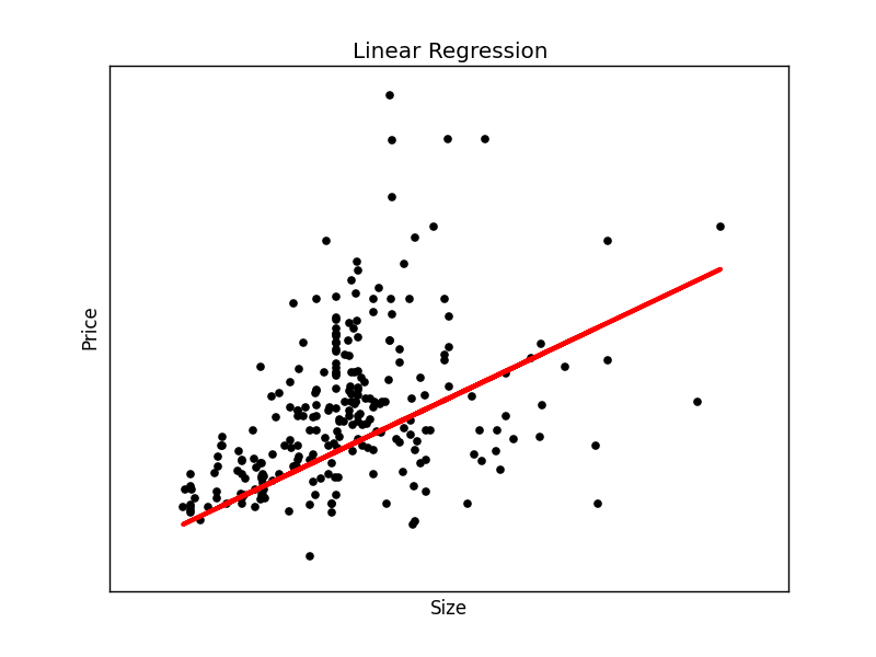
We have created the two datasets and have the test data on the screen. We can continue to create the best fit line:
# Create linear regression object regr = linear_model.LinearRegression() # Train the model using the training sets regr.fit(X_train, Y_train) # Plot outputs plt.plot(X_test, regr.predict(X_test), color='red',linewidth=3) |
This will output the best fit line for the given test data.
To make an individual prediction using the linear regression model:
print( str(round(regr.predict(5000))) ) |
Supervised Learning
Supervised learning algorithms are a type of Machine Learning algorithms that always have known outcomes. Briefly, you know what you are trying to predict.
Related Courses:
Supervised Learning Phases
All supervised learning algorithms have a training phase (supervised means ‘to guide’). The algorithm uses training data which is used for future predictions.
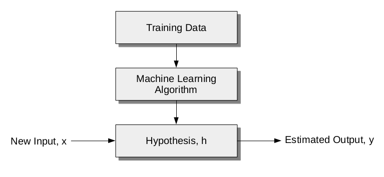
The supervised learning process always has 3 steps:
- build model (machine learning algorithm)
- train mode (training data used in this phase)
- test model (hypothesis)
Examples
In Machine Learning, an example of supervised learning task is classification. Does an input image belong to class A or class B?
A specific example is ‘face detection’. The training set consists of images containing ‘a face’ and ‘anything else’. Based on this training set a computer may detect a face (more similar to features from one set compared to the other set).
Application of supervised learning algorithms include:
- Financial applications (algorithmic trading)
- Bioscience (detection)
- Pattern recognition (vision and speech)