svm python

A common task in Machine Learning is to classify data. Given a data point cloud, sometimes linear classification is impossible. In those cases we can use a Support Vector Machine instead, but an SVM can also work with linear separation.

Related Course:

• Machine Learning Intro for Python Developers

Dataset
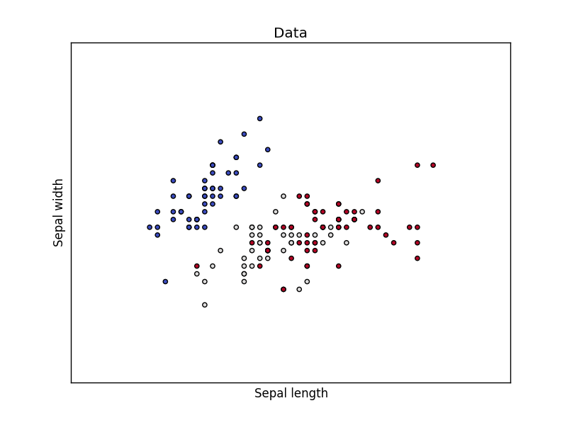
We loading the Iris data, which we’ll later use to classify. This set has many features, but we’ll use only the first two features:

• sepal length
• sepal width

The code below will load the data points on the decision surface.

import matplotlib
matplotlib.use('GTKAgg')

import numpy as np
import matplotlib.pyplot as plt
from sklearn import svm, datasets

# import some data to play with
iris = datasets.load_iris()
X = iris.data[:, :2]  # we only take the first two features.
y = iris.target
h = .02  # step size in the mesh

# create a mesh to plot in
x_min, x_max = X[:, 0].min() - 1, X[:, 0].max() + 1
y_min, y_max = X[:, 1].min() - 1, X[:, 1].max() + 1
xx, yy = np.meshgrid(np.arange(x_min, x_max, h),
np.arange(y_min, y_max, h))

# Plot also the training points
plt.scatter(X[:, 0], X[:, 1], c=y, cmap=plt.cm.coolwarm)
plt.xlabel('Sepal length')
plt.ylabel('Sepal width')
plt.xlim(xx.min(), xx.max())
plt.ylim(yy.min(), yy.max())
plt.xticks(())
plt.yticks(())
plt.title('Data')
plt.show()

Support Vector Machine Example
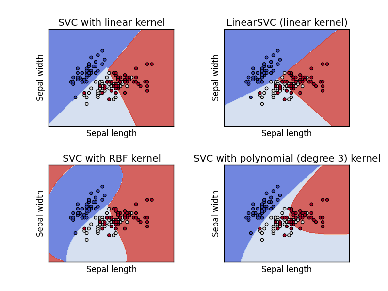
Separating two point clouds is easy with a linear line, but what if they cannot be separated by a linear line?

In that case we can use a kernel, a kernel is a function that a domain-expert provides to a machine learning algorithm (a kernel is not limited to an svm).

The example below shows SVM decision surface using 4 different kernels, of which two are linear kernels.

import matplotlib
matplotlib.use('GTKAgg')

import numpy as np
import matplotlib.pyplot as plt
from sklearn import svm, datasets

# import some data to play with
iris = datasets.load_iris()
X = iris.data[:, :2]  # we only take the first two features. We could
# avoid this ugly slicing by using a two-dim dataset
y = iris.target

h = .02  # step size in the mesh

# we create an instance of SVM and fit out data. We do not scale our
# data since we want to plot the support vectors
C = 1.0  # SVM regularization parameter
svc = svm.SVC(kernel='linear', C=C).fit(X, y)
rbf_svc = svm.SVC(kernel='rbf', gamma=0.7, C=C).fit(X, y)
poly_svc = svm.SVC(kernel='poly', degree=3, C=C).fit(X, y)
lin_svc = svm.LinearSVC(C=C).fit(X, y)

# create a mesh to plot in
x_min, x_max = X[:, 0].min() - 1, X[:, 0].max() + 1
y_min, y_max = X[:, 1].min() - 1, X[:, 1].max() + 1
xx, yy = np.meshgrid(np.arange(x_min, x_max, h),
np.arange(y_min, y_max, h))

# title for the plots
titles = ['SVC with linear kernel',
'LinearSVC (linear kernel)',
'SVC with RBF kernel',
'SVC with polynomial (degree 3) kernel']

for i, clf in enumerate((svc, lin_svc, rbf_svc, poly_svc)):
# Plot the decision boundary. For that, we will assign a color to each
# point in the mesh [x_min, x_max]x[y_min, y_max].
plt.subplot(2, 2, i + 1)
plt.subplots_adjust(wspace=0.4, hspace=0.4)

Z = clf.predict(np.c_[xx.ravel(), yy.ravel()])

# Put the result into a color plot
Z = Z.reshape(xx.shape)
plt.contourf(xx, yy, Z, cmap=plt.cm.coolwarm, alpha=0.8)

# Plot also the training points
plt.scatter(X[:, 0], X[:, 1], c=y, cmap=plt.cm.coolwarm)
plt.xlabel('Sepal length')
plt.ylabel('Sepal width')
plt.xlim(xx.min(), xx.max())
plt.ylim(yy.min(), yy.max())
plt.xticks(())
plt.yticks(())
plt.title(titles[i])

plt.show()

Download Examples and Course

Next